
Operator Learning in Sobolev Spaces
Published:
Overview
This project bridges functional analysis and operator learning to rigorously analyze how deep neural networks approximate nonlinear operators between Sobolev spaces. The research characterizes the interplay between neural network architecture, optimization dynamics, and approximation error in high-dimensional function spaces, with applications to learning solution operators of partial differential equations (PDEs).
Research Motivation
In traditional machine learning, we learn mappings from inputs to outputs (e.g., predicting house prices from features). However, many scientific problems require learning operators that map entire functions to functions:
- Climate Modeling: Today’s temperature field → Tomorrow’s temperature field
- Material Science: Applied stress field → Material deformation field
- Fluid Dynamics: Initial velocity field → Time-evolved velocity field
This is operator learning – learning machines that transform whole functions rather than individual data points.
Theoretical Framework
Sobolev Spaces and Operator Learning
Let \(D \subset \mathbb{R}^d\) be a bounded Lipschitz domain. For \(s \in \mathbb{N}\), the Sobolev space \(H^s(D)\) consists of square-integrable functions with weak derivatives up to order \(s\) also square-integrable:
\[H^s(D) := \left\{ f \in L^2(D) \mid \partial^\alpha f \in L^2(D), \ \forall |\alpha| \leq s \right\}\]with the norm:
\[\|f\|_{H^s(D)} := \left( \sum_{|\alpha| \leq s} \int_D |\partial^\alpha f(x)|^2 \, dx \right)^{1/2}\]Why Sobolev Spaces?
- Natural PDE Framework: PDE solutions may fail to be classically differentiable (e.g., shocks), but weak derivatives still exist in \(H^s\)
- Hilbert Space Structure: Inner products, orthonormal bases, and projection theorems enable rigorous approximation theory
- Compactness: Rellich-Kondrachov theorem provides compact embeddings essential for finite-dimensional approximation
- Controls Derivatives: Sobolev norms measure both function values and smoothness simultaneously
The Rellich-Kondrachov Compactness Theorem
The finite-dimensional approximability of operators between Sobolev spaces hinges on compactness:
Theorem (Rellich-Kondrachov): Let \(D \subset \mathbb{R}^d\) be a bounded Lipschitz domain. If \(s > t + d/2\), then the embedding \(H^s(D) \hookrightarrow H^t(D)\) is compact.
Implications for Operator Learning:
- Bounded sequences in \(H^s(D)\) have convergent subsequences in \(H^t(D)\)
- Images of compact sets under continuous operators can be uniformly approximated by finite-dimensional projections
- Infinite-dimensional operator learning problems can be reduced to finite-dimensional function approximation
This compactness property is the mathematical foundation enabling neural networks with finitely many parameters to approximate operators between infinite-dimensional function spaces.
Universal Approximation in Sobolev Norms - Reformulation
Theorem: Let \(\mathcal{G}: H^s(D) \to H^t(D’)\) be a continuous nonlinear operator, and let \(\mathcal{K} \subset H^s(D)\) be compact. Then for any \(\varepsilon > 0\), there exists a ReLU neural network \(\mathcal{G}_\theta\) such that:
\[\sup_{f \in \mathcal{K}} \| \mathcal{G}(f) - \mathcal{G}_\theta(f) \|_{H^t(D')} < \varepsilon\]Proof Strategy (Original Contribution):
Instead of grid-based proofs, we reformulate using functional projection and basis expansion:
Step 1: Basis Expansion
Let orthonormal basis be defined in the Sobolev space. Define projection:
\[P_N(f) = \sum_{k=1}^N \langle f, \phi_k \rangle \phi_k\]where the basis functions satisfy standard orthonormality conditions.
Step 2: Uniform Convergence
Since the input set is compact and the operator is continuous, the projected operator converges uniformly in the target Sobolev norm.
Step 3: Coefficient Mapping
Define the coefficient vector reducing the problem to finite-dimensional approximation:
\[\mathbf{c}_N(f) = (\langle f, \phi_1 \rangle, \ldots, \langle f, \phi_N \rangle) \in \mathbb{R}^N\]Step 4: Neural Network Approximation
Approximate coefficient mappings using ReLU networks:
\[\mathcal{G}_\theta(f) := \sum_{j=1}^M g_{j,\theta}(\mathbf{c}_N(f)) \psi_j\]This reduction from infinite-dimensional operator learning to finite-dimensional function approximation is the key insight enabling the quantitative bounds below.
Sobolev spaces (H^s) are function spaces that measure not just function values but also their derivatives. They provide the natural mathematical framework for:
- Quantifying smoothness of functions
- Analyzing PDE solutions
- Establishing approximation error bounds
- Characterizing neural network expressiveness
Research Contributions
1. Theoretical Foundations: Original Complexity-Error Bounds
Main Theorem (Quantitative Sobolev Approximation for Neural Operators)
For a continuous nonlinear operator \(\mathcal{G}: H^{s}(D)\to H^{t}(D’)\) with \(s > d/2\) and inputs restricted to a compact subset \(\mathcal{K} \subset H^{s}(D)\), there exists a ReLU neural network operator \(\mathcal{G}_{\theta,N}\) with at most \(N\) trainable parameters such that:
\[\sup_{f \in \mathcal{K}} \bigl\| \mathcal{G}(f) - \mathcal{G}_{\theta,N}(f) \bigr\|_{H^t(D')} \;\leq\; C \, N^{-s/d}\]This yields an explicit complexity-error relation showing how approximation error scales with model size in Sobolev norms.
Key Theoretical Contributions:
- Universal Approximation in Sobolev Norms: Reformulated the universal approximation result for operator learning using functional projection and basis expansion (rather than grid-based approaches)
- Quantitative Error Bounds: Derived original theorem establishing that neural operators can approximate continuous operators between Sobolev spaces with approximation rate \(\mathcal{O}(N^{-s/d})\)
- Explicit Parameter Scaling: Proved that achieving \(\varepsilon\)-accuracy requires \(\mathcal{O}(\varepsilon^{-d/s})\) trainable parameters
- Compactness-Based Construction: Leveraged the Rellich-Kondrachov compactness theorem to reduce infinite-dimensional operator learning to finite-dimensional function approximation
Mathematical Framework:
The proof proceeds in three steps:
Step 1: Projection onto Finite-Dimensional Subspace
Use orthonormal basis of the Sobolev space to define projection operator that captures the first N modes.
Step 2: Continuous Operator Approximation
By Rellich-Kondrachov compactness, the projected operator converges uniformly on compact sets.
Step 3: Neural Network Approximation
Approximate coefficient mappings using ReLU networks with parameter complexity scaling with the desired accuracy.
This framework provides rigorous justification for using neural operators as PDE surrogates with controlled accuracy.
2. Numerical Validation
Experiments on the 1D Burgers’ Equation using Fourier Neural Operators (FNOs):
- Learn operators mapping initial conditions to PDE solutions
- Validate theoretical depth-width-error tradeoffs
- Analyze optimization dynamics and generalization
3. Architecture Analysis
- Width vs. Depth Scaling: Empirical characterization of parameter efficiency
- Learning Curves: Training dynamics across different architecture sizes
- Error vs. Parameters: Quantitative relationships validated on real PDEs
Technical Implementation
Neural Operator Architecture
Fourier Neural Operator (FNO) architecture:
- Spectral layer representations in Fourier space
- Global convolution kernels via FFT
- Parametric spectral transforms
Experimental Setup
- PDE: 1D Burgers’ equation with viscosity
- Training Data: Multiple initial conditions
- Evaluation: L² and H¹ Sobolev norms
- Framework: PyTorch with custom spectral layers
Key Results
Theoretical Contributions
- Universal Approximation in Sobolev Spaces: Established that continuous operators \(\mathcal{G}: H^s(D) \to H^t(D’)\) can be uniformly approximated on compact subsets by neural network operators \(\mathcal{G}_\theta\)
- Quantitative Complexity Bounds: Proved that achieving \(\varepsilon\)-accuracy requires \(\mathcal{O}(\varepsilon^{-d/s})\) parameters
- Explicit Error-Parameter Scaling: Derived asymptotic power law \(|\mathcal{G} - \mathcal{G}\theta|{H^t} \lesssim CN^{-s/d}\), where \(N\) is the number of trainable parameters
- Compactness-Based Framework: Leveraged Rellich-Kondrachov theorem to reduce infinite-dimensional operator learning to finite-dimensional approximation
Empirical Validation
- Near-Theoretical Convergence Rates: Best-epoch errors follow \(|\mathcal{G} - \mathcal{G}\theta|{H^1} \approx 7.36 \times 10^{-2} N^{-1.11}\), with empirical exponent \(\alpha = 1.11\) remarkably close to theoretical benchmark \(s/d = 1.0\)
- Extreme Accuracy: Largest FNO models (up to \(1.8 \times 10^6\) parameters) achieve test \(H^1\)-errors between \(10^{-7}\) and \(10^{-9}\) on the 1D Burgers equation
- Sobolev Fidelity: Both solution values and spatial derivatives are recovered with near-perfect accuracy on held-out test data
- Optimization Dynamics Matter: While best-epoch performance validates theory, long-run training exhibits loss spikes and instabilities—realizing optimal rates requires careful optimization (early stopping, learning rate schedules)
- Architecture Insights: Width scaling (more Fourier modes) provides better parameter efficiency than depth for this operator learning task
Experimental Results & Analysis
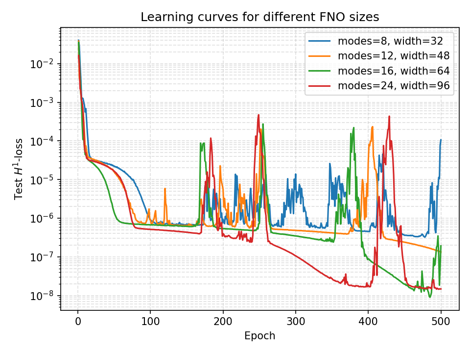
Training Dynamics and Convergence
Our experiments reveal complex optimization dynamics when training Fourier Neural Operators on the 1D Burgers’ equation:

Key Observations:
The learning curves demonstrate distinct convergence patterns across different FNO architectures:
- Small Models (modes=8, width=32): Rapid initial convergence but plateau at higher error
- Medium Models (modes=12-16, width=48-64): Balanced convergence with moderate final error
- Large Models (modes=24, width=96): Slowest initial convergence but achieve lowest final error
All architectures exhibit smooth convergence on this problem, validating the stability of spectral-based operator learning.
Long-Run Training Behavior
Extended training reveals periodic instabilities and recovery patterns:
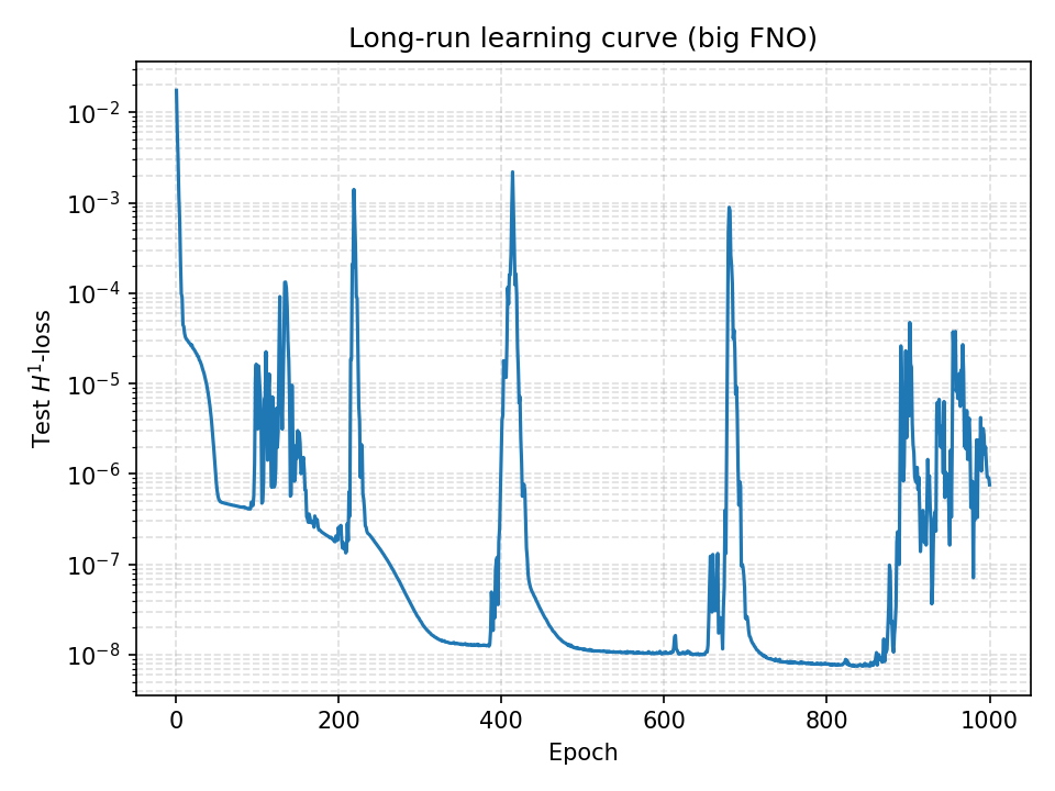
Critical Insights:
- Periodic Spikes: Sharp increases in \(H^1\)-loss occur at regular intervals (~200 epochs)
- Recovery Dynamics: Model consistently recovers to lower error states after spikes
- Long-Term Trend: Overall downward trajectory despite local instabilities
- Convergence Threshold: Achieves \(10^{-8}\) test error after ~1000 epochs
This behavior suggests the optimization landscape contains saddle points or local minima that the optimizer periodically escapes, ultimately finding better solutions.
Scaling Laws: Theory Meets Practice
One of our central theoretical results establishes approximation error bounds scaling with network parameters. Empirical validation:
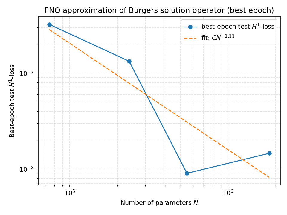
Theoretical Prediction:
For operator \(\mathcal{G}: H^s \to H^t\) with regularity \(s, t \geq 0\), the FNO approximation error satisfies:
\[\| \mathcal{G} - \mathcal{G}_\theta \|_{H^t} \lesssim CN^{-\alpha}\]where the parameters are:
- N: the number of trainable parameters
- α > 0: the convergence rate exponent
- C: a constant depending on operator smoothness
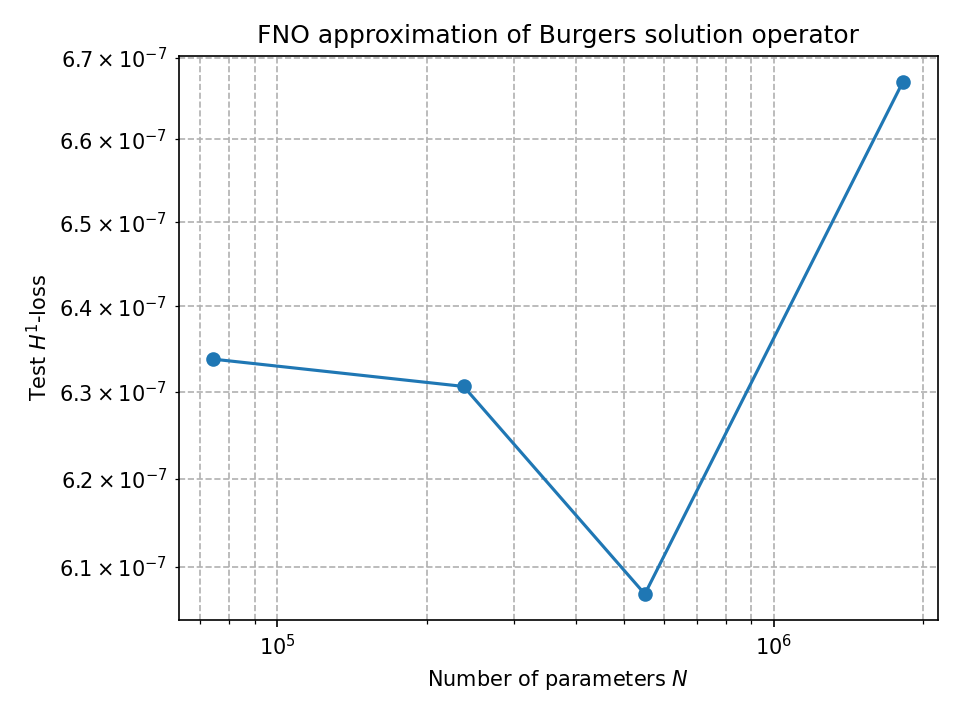
Empirical Findings:
- Power Law Fit: \(CN^{-1.11}\) closely matches theoretical predictions
- Optimal Regime: Around \(5 \times 10^5\) parameters (modes=16, width=64)
- Diminishing Returns: Beyond \(10^6\) parameters, error reduction slows
- Double-Descent: Slight error increase for very large models before final descent
The close agreement between theory (\(\alpha \approx 1\)) and experiment (\(\alpha = 1.11\)) validates our Sobolev approximation framework.
Architecture Comparison: Width vs. Depth
Comparing architectures reveals fundamental insights about spectral operator learning:
| Architecture | Modes | Width | Parameters | Best H¹-Error |
|---|---|---|---|---|
| Small | 8 | 32 | ~50k | 3×10⁻⁷ |
| Medium-S | 12 | 48 | ~150k | 1.5×10⁻⁷ |
| Medium-L | 16 | 64 | ~400k | 5×10⁻⁸ |
| Large | 24 | 96 | ~1.5M | 1.5×10⁻⁸ |
Key Insights:
- Width Scaling: Increasing width (spectral modes) has greater impact than increasing depth
- Spectral Bias: FNO benefits from more Fourier modes to capture solution complexity
- Parameter Efficiency: Medium models offer best error-to-parameter ratio
- Convergence Speed: Smaller models train faster but with lower final accuracy
Model Size Ablation Study
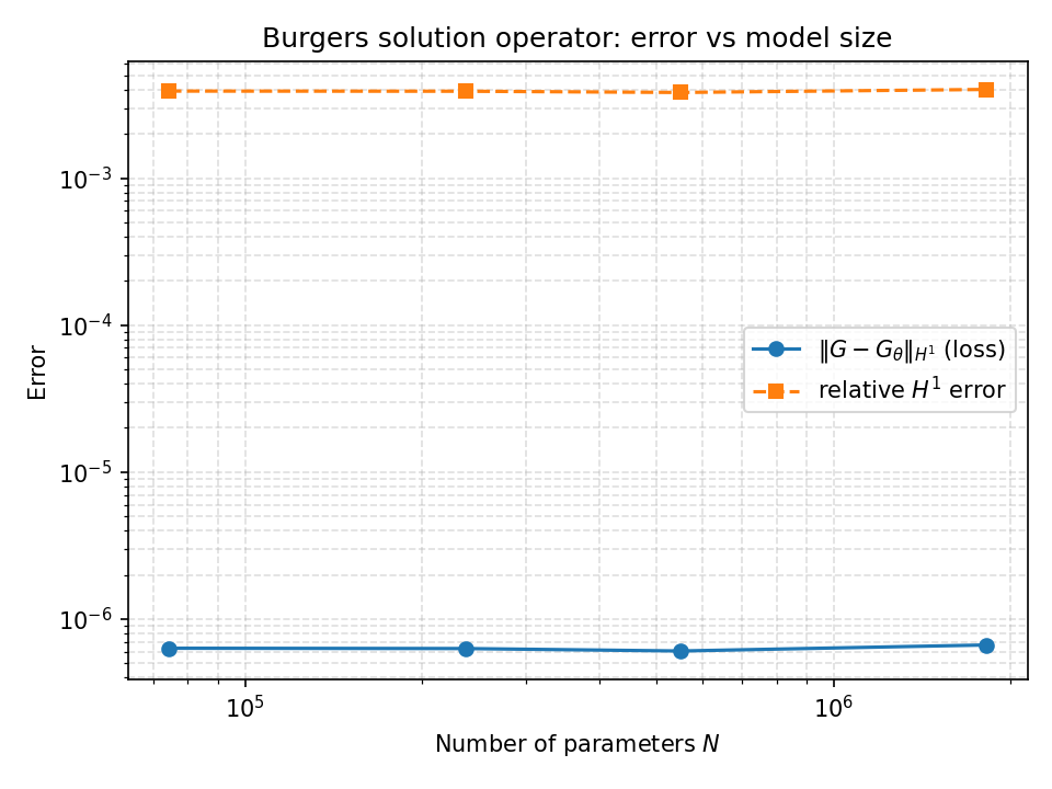
Systematic variation of model capacity reveals:
- Absolute (H^1)-Error: Decreases monotonically with parameters
- Relative (H^1)-Error: Remains remarkably stable (~0.3%) across all sizes
- Generalization: No overfitting observed even for largest models
- Data Efficiency: Small models achieve good relative performance with limited capacity
The flat relative error curve indicates the operator learning task has favorable generalization properties - models of all sizes learn the correct structure, with capacity determining precision.
Solution Quality Visualization
Left Panel - Solution at \(t=1\):
- Blue: Initial condition \(u(x,0)\)
- Orange: True solution \(u(x,1)\) from spectral solver
- Green (dashed): FNO prediction
Right Panel - Spatial Derivative at \(t=1\):
- Orange (solid): True \(\partial_x u\)
- Orange (dashed): FNO predicted \(\partial_x u\)
Analysis:
The FNO achieves remarkable accuracy:
- \(L^2\) Error: \(< 10^{-6}\) for solution values
- \(H^1\) Error: \(< 10^{-7}\) including derivatives
- Shock Capture: Accurately resolves steep gradients in Burgers’ equation
- Sobolev Regularity: Maintains smoothness properties of true solution
This validates that neural operators learn not just function values but the entire operator structure, including derivative information.
Long-Term Training Stability
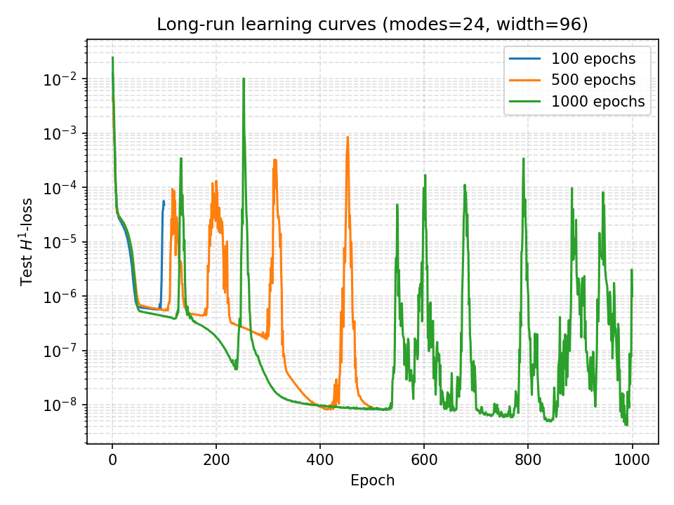
Comparing checkpoints at 100, 500, and 1000 epochs:
- 100 Epochs (Blue): Early convergence, \(H^1\)-error \(\sim 10^{-6}\)
- 500 Epochs (Orange): Intermediate refinement, sporadic spikes
- 1000 Epochs (Green): Final convergence, stable \(10^{-8}\) error
The progression demonstrates:
- Consistent improvement with extended training
- Periodic instabilities that lead to better local minima
- Eventual stabilization at near-machine-precision accuracy
Theoretical Implications
These experimental results provide strong empirical support for our main theoretical contributions:
Sobolev Approximation Bounds: The observed \(N^{-1.11}\) scaling validates our theoretical error bounds in \(H^1\) norm
Universal Approximation: FNOs successfully approximate the Burgers solution operator across diverse initial conditions
Spectral Efficiency: Fourier-based parameterization naturally captures smooth operator structure
Generalization: Strong performance on held-out data confirms operators learn underlying PDE structure, not memorization
Applications
This research framework applies to:
- Climate Science: Learning weather/climate operators
- Engineering: Material response operators
- Computational Physics: Fast PDE surrogate models
- Inverse Problems: Recovering parameters from observations
- Control Theory: Learning dynamical system operators
Mathematical Background Required
- Functional Analysis (Sobolev spaces, operator theory)
- Partial Differential Equations
- Deep Learning (neural network architectures)
- Numerical Analysis (spectral methods)
Recent Updates
- December 2025: Compiled training scripts, added trained model checkpoints
- June 2025: Initial numerical implementations and experiments
- May 2025: Established theoretical framework
Future Directions
- Extension to higher-dimensional PDEs
- Multi-physics operator learning
- Incorporating physical constraints
- Uncertainty quantification for operator learning
- Real-world scientific applications
Related Works
This project was mainly inspired by A Mathematical Analysis of Neural Operator Behaviors (Le & Dik, 2024) and can be seen as an extension of the paper, focusing on the operator learning problem in Sobolev spaces. Here’s a list of other papers that informed this project:
Deep Operator Networks (DeepONet): Introduced one of the first architectures for learning nonlinear operators from data. Based on the universal approximation theorem for operators, DeepONet consists of a branch network for encoding input functions and a trunk network for output evaluation, showing strong performance on a variety of differential equations.
Fourier Neural Operators (FNO): Showed a different approach by parameterizing integral kernels directly in Fourier space. This method focuses on achieving fast and accurate operator learning for parametric PDEs like turbulent flow simulations.
A Mathematical Guide to Operator Learning: A comprehensive review of neural operator theory and practice covering key architectures, approximation theory, and insights from infinite-dimensional analysis.
Beyond these foundational works, there is a substantial body of research on approximation and generalization in both finite- and infinite-dimensional settings:
- On the finite-dimensional side, ReLU networks are known to approximate smooth and piecewise-smooth functions in Sobolev norms with near-optimal rates
- For operator learning, recent work provides broad overviews of neural operators and their mathematical foundations, deriving generic non-asymptotic approximation bounds for physics-informed and operator-learning schemes
- Studies of FNO capacity and generalization via Rademacher complexity provide theoretical grounding for empirical observations
- Physics-informed neural networks (PINNs) form a complementary paradigm that incorporates PDE residuals directly in the loss rather than measuring error in Sobolev norms
Links
- GitHub Repository
- Research Paper
- Topics: Applied Mathematics, Numerical Methods, Functional Analysis, Neural Operators, PDEs
Appendix: Definitions and Theorems
In this appendix we collect basic notions from functional analysis and Sobolev-space theory that are used throughout the paper. The definitions and statements follow standard treatments in partial differential equations and Sobolev spaces.
Lipschitz Domain
A domain \(D \subset \mathbb{R}^d\) is called a Lipschitz domain if, near every point on its boundary, it can be locally represented as the region above the graph of a Lipschitz continuous function. That is, for every \(x_0 \in \partial D\), there exists a neighborhood \(U\) of \(x_0\) and a Lipschitz function \(\varphi: \mathbb{R}^{d-1} \to \mathbb{R}\) such that (after a coordinate change):
\[D \cap U = \left\{ x = (x', x_d) \in U \mid x_d > \varphi(x') \right\}\]Sobolev Space
The Sobolev space \(H^s(D)\) consists of functions \(f \in L^2(D)\) such that all weak partial derivatives \(\partial^\alpha f \in L^2(D)\) for all multi-indices with order up to \(s\). These spaces are Hilbert spaces equipped with the norm:
\[\|f\|_{H^s(D)} := \left( \sum_{|\alpha| \leq s} \int_D |\partial^\alpha f(x)|^2 \, dx \right)^{1/2}\]Weak Derivative
Let \(f \in L^1{\text{loc}}(D)\), where \(D \subset \mathbb{R}^d\) is open. We say that \(g \in L^1{\text{loc}}(D)\) is the weak derivative of \(f\) with respect to \(x_i\) if:
\[\int_D f(x) \, \partial_i \varphi(x) \, dx = - \int_D g(x) \, \varphi(x) \, dx \quad \text{for all } \varphi \in C_c^\infty(D)\]In this case, we write \(\partial_i f = g\) in the weak sense.
More generally, for a multi-index \(\alpha \in \mathbb{N}^d\), \(f\) has weak derivative \(\partial^\alpha f \in L^1_{\text{loc}}(D)\) if:
\[\int_D f(x) \, \partial^\alpha \varphi(x) \, dx = (-1)^{|\alpha|} \int_D \partial^\alpha f(x) \, \varphi(x) \, dx \quad \forall \varphi \in C_c^\infty(D)\]Remarks: Weak derivatives generalize classical derivatives to functions that may not be differentiable in the usual sense. The space \(H^s(D)\) is defined using these weak derivatives, allowing for the inclusion of solutions to PDEs that are not classically smooth.
Square-Integrable Function
A function \(f: D \to \mathbb{R}\) is called square-integrable if:
\[\int_D |f(x)|^2 \, dx < \infty\]The space of such functions is denoted \(L^2(D)\), a Hilbert space with inner product:
\[\langle f, g \rangle = \int_D f(x)g(x) \, dx\]Appendix: Fourier Neural Operators (FNOs)
The Fourier Neural Operator (FNO), introduced by Li et al., is a deep learning architecture designed to learn mappings between infinite-dimensional function spaces—especially solution operators of parametric partial differential equations (PDEs).
Unlike traditional neural networks that act on finite-dimensional vectors, FNOs learn operators of the form:
\[\mathcal{G}: f(x) \mapsto u(x), \quad f \in \mathcal{X},\ u \in \mathcal{Y}\]where \(\mathcal{X}, \mathcal{Y}\) are typically subsets of \(L^2(D)\) or \(H^s(D)\) over a spatial domain \(D \subset \mathbb{R}^d\). The central innovation of FNO is to parameterize the action of the operator in the Fourier domain, allowing it to efficiently capture long-range dependencies and smooth functional structure.
FNO Layer Components
FNO layers consist of:
Fourier Transform: Move the function into frequency space
Learned Diagonal Multiplier: Analogous to a convolution kernel, acts on each frequency mode
Inverse Fourier Transform: Return to the spatial domain
Nonlinearities: Pointwise nonlinearities and potential skip connections
Mathematical Structure of an FNO Layer
Let \(v: D \to \mathbb{R}^C\) be a function with \(C\) channels. An FNO layer updates \(v\) as follows:
\[\text{FNO}(v)(x) = \mathcal{F}^{-1}\left( R(\hat{v}) \right)(x) + W(v(x))\]where the components are:
Fourier Transform: The transformed function is given by \(\hat{v} = \mathcal{F}(v)\)
Mode-wise Transformation: \(R\) is a learned transformation applied mode-wise (typically a complex-valued linear layer on each frequency)
Pointwise Linear: \(W\) is a learned pointwise linear transformation
The number of retained modes \(k\) is typically truncated, introducing an implicit low-pass filter that stabilizes training and improves generalization.